Words are (not) particles!

Last time I went through the first few equations of the word2vec paper (Distributed Representations of Words and Phrases and their Compositionality) and thought through how the equation for the probability of an output word, given the input word, compared to another formula of the same form: the Boltzmann Distribution. This time, I’ll finish the paper, which requires me to leave behind the particle analogy almost completely.

Our goal is to figure out how to actually calculate this equation: 

\[p(w_O \vert w_I) = \frac{e^{ \left( {v'}_{w_O}^\top v_{w_I} \right) }}{\sum_{w=1}^W e^{\left( {v'}_w^\top v_{w_I} \right) }}\]

It’s the denominator here that’s costly. To do the maximization of the average log probability properly, we’d have to calculate $ \nabla p(w_O \vert w_I) $ and that’s going to be hard when you have to do it for every word in the vocabulary, which can be tens of thousands of words.

The next three sections of the paper are about ways to approximate this equation: hierarchical softmax, noise contrastive estimation, and negative sampling.

TREES:

I admit, this part of the paper threw me. Physicists tend to approximate in ways that yield a more tractable closed form solution. Computer scientists, though, tend to approximate in ways that yield a more tractable computation.

So when the next part of the paper suggested that we replace this equation with a binary tree representation (the hierarchical softmax), my brain made the sound a fork makes when it gets stuck in the garbage disposal. This is a deeply clever thing to do that would never have occurred to me and it totally broke my brain for a bit.

Here are two (1 and 2) great online resources that I used to understand most of the rest of this paper.

The way this works is like this. The regular softmax equation can be thought of as tree of depth 1, where every word in the vocabulary is a leaf node.

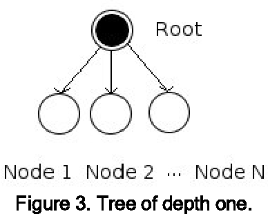
The problem here is that you then have to normalize over every leaf, which is expensive. So instead, we reformulate the softmax equation as a binary tree, which takes the number of computations we need to do from $O(W) $ to $O(\log_2 W) $.

Something like this:

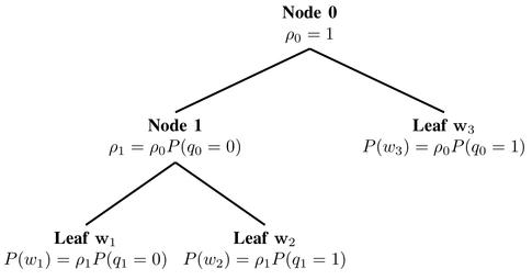
Of course, you have to figure out how to construct this tree, which is a literature deep dive all on its own. For this paper, they’re using something called a Huffman tree, which is a totally well-known thing if you are a computer science person. (I am not.) My physics intuition starts to break down here, as I did not encounter this representation of data much in my coursework. So, it turns out, that perhaps words and particles are different after all.

SAMPLING

The next two approximations for the softmax equation that the paper mentions  are based on importance sampling. To understand these sections, it’s important to remember that our goal is to maximize the average log probability of an input word, given an output word. Something like this:

\[J_{\theta} =  \log \frac{e^{ \left( {v'}_{w_O}^\top v_{w_I} \right) }}{\sum_{w=1}^W e^{\left( {v'}_w^\top v_{w_I} \right) }}\]

Here we are using $ \theta $ to represent the parameters of the model. Then in order to do that maximization, we will need to calculate the gradient of our loss function $ \nabla_{\theta} J_{\theta} $.

We do some computation, set \(\mathcal{E} = {v'}_w^\top v_{w_I}\), and end up with the following (all the steps are in the second reference, above):

\[\nabla_{\theta} J_{\theta} = \nabla_{\theta}\mathcal{E}(w) - \sum_{i=1}^W P(w_i)\nabla_{\theta}\mathcal{E}(w_i)\]

The first term in the equation can be thought of as positive reinforcement for the target word. The second term can be thought of as negative reinforcement for all the other words, weighted by their probability. Another way to think about the second term in the equation is as the expectation value of the gradient of $\mathcal{E}$ for all words in the vocabulary.

\[\sum_{i=1}^W p(w_i) \nabla_{\theta}\mathcal{E} (w_i) = \mathbb{E}_{w_i \approx P}[\nabla_{\theta} \mathcal{E}(w_i)].\]

So far this is all exact. We haven’t actually approximated the softmax by anything. Now, we want to approximate the expected value, $\mathbb{E}$, in a way that makes this easier to compute, which brings us to sampling based based approaches.

The idea here is that you can approximate the expected value of a probability distribution $P$ by taking means of random samples from that distribution. Here lies the catch-22. In order to sample from the distribution $P$ you have to compute the distribution, which is the computation we are trying to avoid.

Instead, we try to find a different distribution $Q$, which is less computationally expensive, but that still approximates $P$  in nice, high-fidelity ways.

Noise Contrastive Estimation is a way of doing just that. You approximate $P$  (the true distribution of all words) with, for example, the unigram distribution of words in your training set. You then compare samples from that distribution with samples from a “noise” data set and train a logistic regression model to distinguish between the “true” and “noise” samples. Frankly, there’s a lot going on with this technique and I’m not the one to explain it all. (Reference 2 above has a beautiful explanation of all of this.)

Even this technique is relatively computationally intensive, so we approximate it again with Negative Sampling. 

This technique assumes that the noise distribution from NCE is the uniform distribution and that we sample the entire vocabulary. There are lots of details to this, but the main thing I learned from this that this only works because we are interested in learning word embeddings, and not doing language modeling.

Interestingly, in this paper they actually use the unigram distribution raised to the 3/4 power for the noise distribution, not the uniform distribution. This seems like a hella random choice to me, but it apparently it works.

The last approximation technique mentioned in the paper is subsampling. As I talked about in the last post, the most frequent (low energy) words provide less information than the rare (high energy) words. The most frequent words (“the”, “an”, “and”) occur many many many times more frequently than the rare words (“mugwump”) and we can correct for that imbalance by subsampling the training set by inverse frequency. Each word in the training set is discarded with probability given by the following formula, where $t$ is chosen via heuristic.

\[P(w_i) = 1 -\sqrt{\frac{t}{f(w_i)}}\]

So, if $f(w_i) » t$, then the fraction under the square root is small and the probability it will get thrown out is close to one. That is, more frequent words get thrown out more often.

THE REST OF THE PAPER

Phew. Now we are through the bits we need to understand the actual results of the paper. They compare the accuracy of the Skip-gram model on a news data set using the three approximation techniques (hierarchical softmax, NCE, and NEG), both with and without the additional subsampling technique.

The hierarchical softmax with subsampling appears to do the best on most of the tasks they examine. It also blows previously published results on word analogy tasks out of the water. Add in the results on the additive compositionality (e.g. “Vietnam + capital = Hanoi”) and you have a deeply impressive, game-changing paper on word embeddings. NBD, right?